👋 Hi! I’m Bibin Wilson. Every Saturday, I publish a deep-dive MLOps edition to help you upskill step by step. If someone forwarded this email to you, you can subscribe here so you never miss an update.
In today’s MLOPS edition, we will cover:
What data preparation is and why it matters.
Who owns this step in a real MLOps team.
Key stages of the data preparation pipeline.
Hands-on execution of data preparation python scripts.
Creating final dataset for model training.
Note: Please read the online version for better reading experience.
📦 DevOps To MLOps Code Repository
All hands-on code for the entire MLOps series will be pushed to the DevOps to MLOps GitHub repository. We will refer to the code in this repository in every edition.
If you are using the repository, please give it a star.
Need for Data Preparation
In the last edition, we looked at the dataset pipeline and ended up with a clean 300MB CSV file (dataset). One row per employee, pulled from HRMS, payroll, and performance systems. If you missed it, read it here first.
Now here is the thing. That 300MB CSV is not ready for training a model yet. It still has problems that need fixing and transformations that need to happen before a machine learning model can learn anything useful from it.
That is exactly what the Data Preparation Pipeline does. It takes our raw dataset, explores it, cleans it up, and converts it into final training and test files that a machine learning model can work with.
Data Preparation Stages
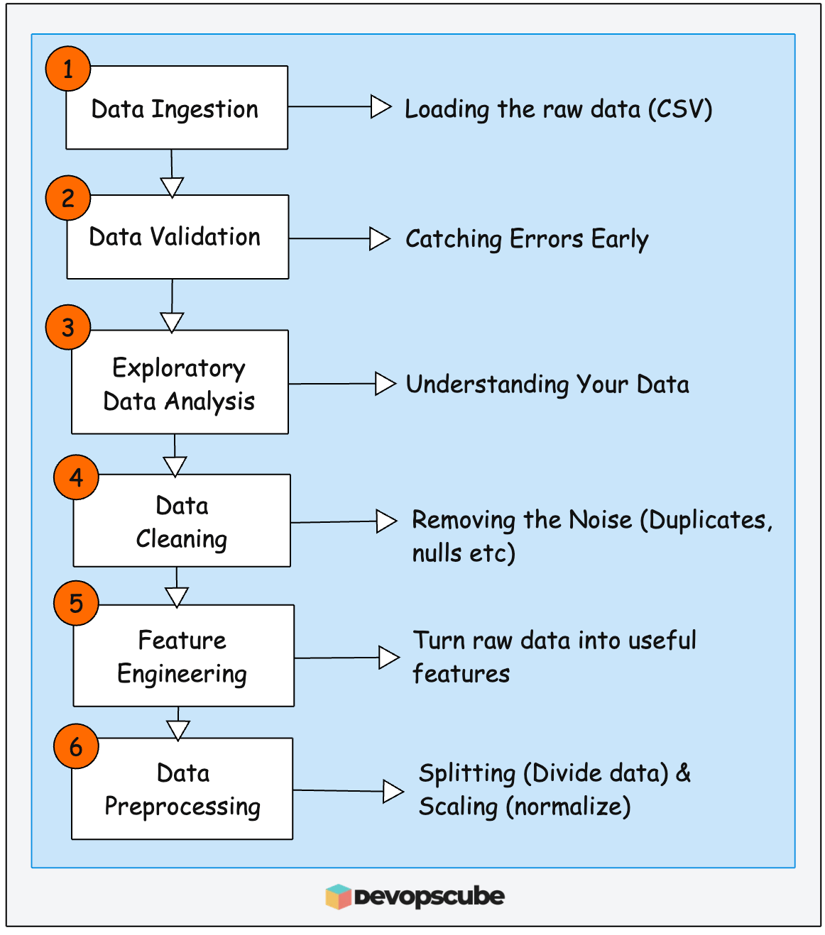
The following image illustrates the data preparation stages in our ML lifecycle. Overall these stages collects data, explore patterns, cleans data and creates useful features.

📌 Important Note Before You Start
You do not need to understand the data science behind these scripts. That is the Data Scientist's job. They write the scripts, they own the logic.
In this edition, I want to do two things.
First, give you a clear mental model of what this pipeline does and who owns each part of it in a real team.
Second, walk you through running it locally on your machine. Not so you become a data scientist, but so you understand exactly what you will be automating later in this series.
What Happens in the Real World
Before we jump into code, let's talk about what this step looks like in an actual enterprise ML project.
In our employee attrition project, the Data Engineering team (Step 1) hands over a versioned 300MB CSV stored in S3 to the Data Science team . That handoff is the starting point for everything in this edition.
Data Preparation is typically owned by Data Scientists, but DevOps/MLOps engineers need to understand it because they will eventually automate and build pipeline for this process.
In production, each of these Python scripts becomes an Airflow task, a Kubeflow pipeline step, or a step in a GitHub Actions workflow. (We will create that pipeline using Kubeflow later in the MLOPS series).
Who Owns What in a Real Team
Before touching any code, let's be clear about who does what in a real enterprise MLOps team. This is important because your job as a DevOps engineer is specific and it is different from what the Data Scientist does.
Team | What They Own | Your Overlap |
|---|---|---|
Data Scientists | Write the Python scripts for all stages. | You run their code. You don't write it. |
Data Engineers | Ensure the upstream CSV arrives in the expected format. | You manage the storage (S3) and access policies they depend on. |
DevOps / MLOps | Provision infrastructure for the Data Science team. Automate and orchestrate the pipeline. Manage environments. Handle failures. Monitor runs. | This is your primary job. |
InfoSec / Compliance | Ensure PII is handled correctly. Audit data access and lineage. | You enforce their policies via IAM roles, encryption, and audit logging. |
Before a Data Scientist writes a single line of code, someone has to set up the environment they work in. That someone is you (Providing notebook environment or managed service like AWS SageMaker Studio, compute with the right sizing, S3 IAM access etc.
Setting Up Your Local Environment
We have pushed every required files and source code into our GitHub repository.
Clone the repository and move into the phase-1-local-dev folder using the following commands.
git clone https://github.com/techiescamp/mlops-for-devops.git

cd mlops-for-devops/phase-1-local-dev
Create and activate virtual environment.
# Mac / Linux
python3 -m venv venv
source venv/bin/activate

# Windows (PowerShell)
python -m venv venv
venv\Scripts\activate
Install project dependencies.
pip install -r requirements.txtOnce that is done, you will see the following project structure.
.
├── datasets
│   └── employee_attrition.csv    ← our 9.5MB raw dataset
├── requirements.txt
└── src
    ├── config
    │   └── paths.py
    └── data_preparation
        ├── 01_ingestion.py
        ├── 02_validation.py
        ├── 03_eda.py
        ├── 04_cleaning.py
        ├── 05_feature_engg.py
        └── 06_preprocessing.py
The src/data_preparation/ folder is where all 6 data preparation steps live and numbered so you always know the order to run them.
datasets/employee_attrition.csv is our raw dataset that we will be working on. It was taken from Kaggle and modified it based on our project requirements.
Why Are We Running This Locally?
You might be thinking, "I'm a DevOps engineer. Running Python scripts manually isn't my job. Why am I doing this?"
That's a fair question. Here is the honest answer.
In Phase 3 of this series, you will automate this entire pipeline on Kubeflow + MLFlow running on Kubernetes. You set up the pipelines and manage the infrastructure. That is your job.
But here is the problem. If you have never run these scripts yourself, you will be automating a black box.
By running it locally, you will understand what each stage does and what can go wrong. Think of it the same way a DevOps engineer understands how a Java app builds before they set up the CI/CD pipeline for it.
Before We Start: Understanding paths.py
Before running any script, there is one file worth understanding first config/paths.py
Every pipeline script in data_preparation folder needs to know two things.
Where to read its input data from
Where to write its output to.
So, instead of hardcoding file paths inside every script, we define them all in one central place paths.py. Every script then imports from this file.
Think of it like a single source of truth for all your file locations. If you ever need to change where a file gets saved, you change it in one place and not in 6 different scripts.
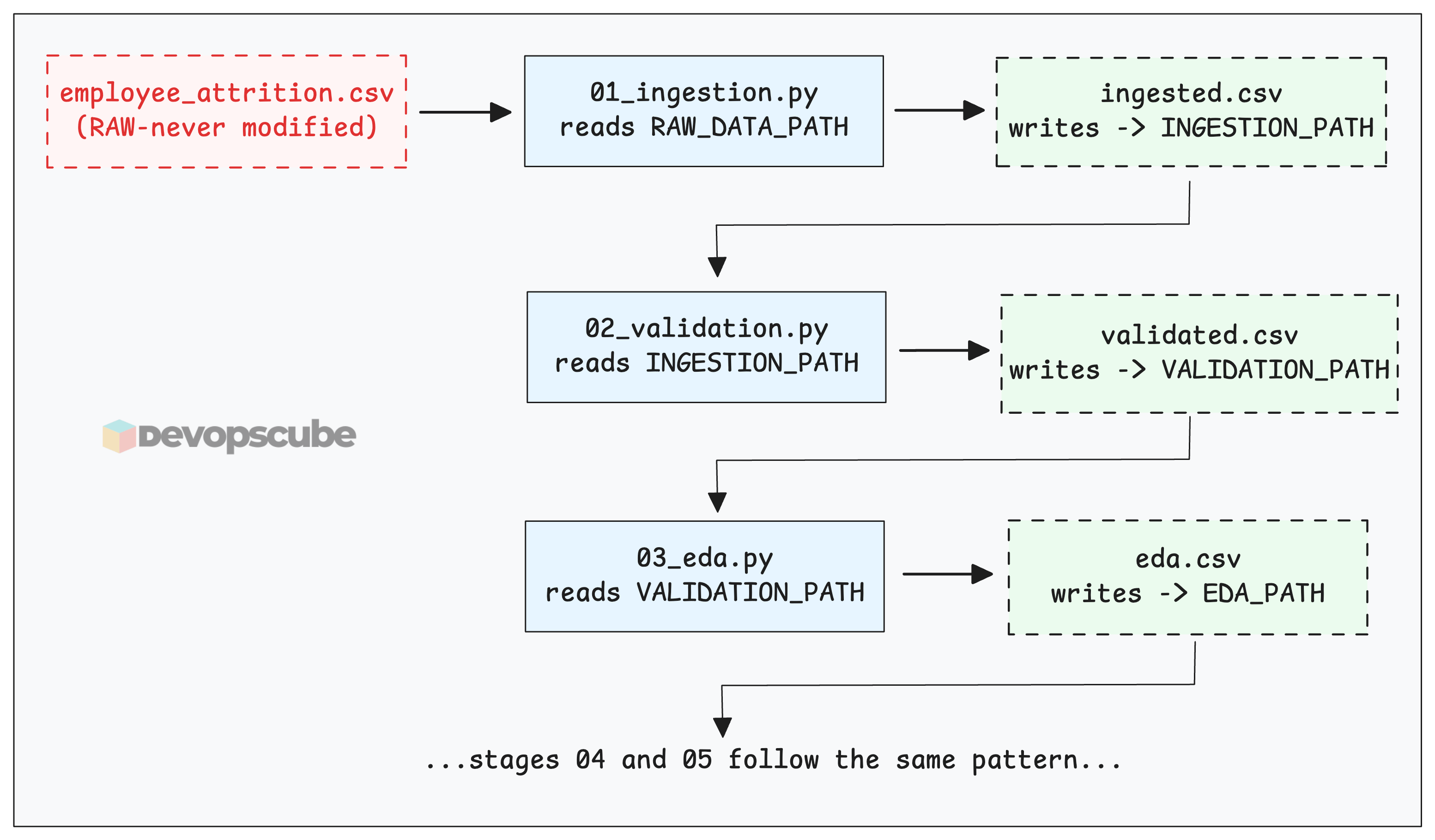
Now here is the important pattern. Every script reads from the previous stage's output and writes to its own output path. The original raw file is never touched after the first read.

Lets understand each stage by practically executing the scripts.
1. Data Ingestion (01_ingestion.py)
This script loads the employee_attrition.csv into memory as a DataFrame. Python's in-memory table structure. Think of a DataFrame as a spreadsheet that lives in RAM.
It then prints a snapshot of first 5 rows, shape (rows × columns), and column data types. So you can confirm the file loaded correctly.
Now lets execute the script.
cd src

python -m data_preparation.01_ingestion
Once executed writes an identical copy to datasets/processed/raw_ingested.csv
Why write the same file? Because every subsequent stage reads from the previous stage's output, never from the original dataset.
2. Data Validation (02_validation.py)
The data we get is not always perfect. It can be inconsistent and have some missing values. So, it is important to check the schema and quality of the dataset, so that errors are caught early instead of breaking the model later.
The script uses pandera to define a schema. Meaning which columns are expected, what data types they must be, and what values are allowed.
For example: the "Age" column must be an integer greater than 18. The "Attrition" column must only contain "Stayed" or "Left". If anything violates the schema, the script raises an error with a detailed failure report.
Lets execute the code.
python -m data_preparation.02_validationYou should see “Data validation successful” message.
🔥 Try This: Break It Deliberately
Open datasets/processed/raw_ingested.csv and change a few values in the "Age" column to empty(null) values. Save and re-run validation again. You will see “Data validation errors found”
3. Exploratory Data Analysis (03_eda.py)
EDA is where the Data Scientist reads the data before making any decisions about it.
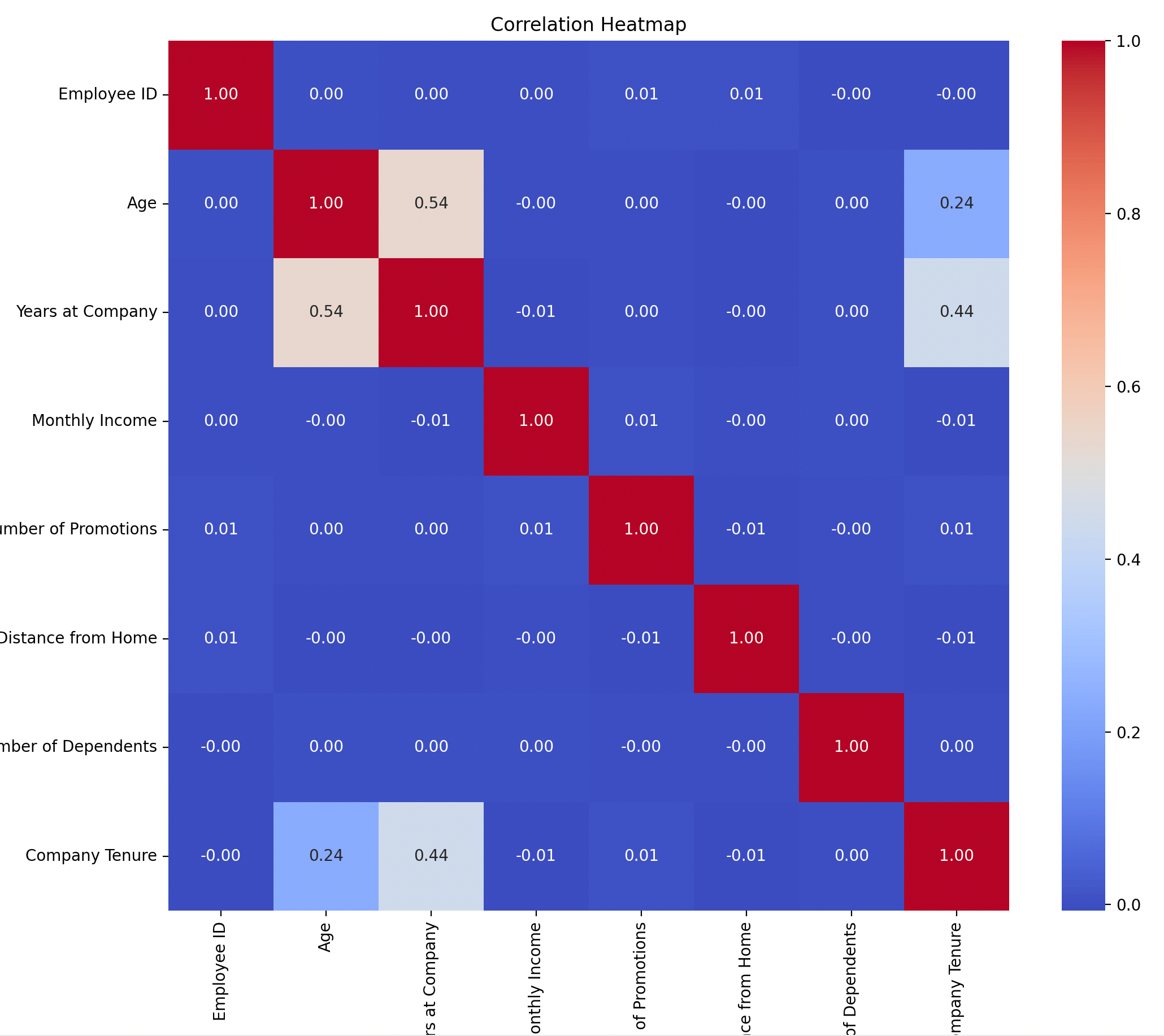
This script generates four charts (age distribution, attrition counts, and a correlation heatmap) using seaborn and matplotlib libraries and prints summary statistics.
When you run the script, chart windows open one by one behind your terminal or on another monitor (Find it). Close each chart to see the next. After the fourth chart, the script writes eda.csv and exits cleanly.
Lets execute it.
python -m data_preparation.03_edaHere is an example Correlation Heatmap generated (chart 4). The Data Scientist uses this to decide what to keep and what to combine in feature engineering.

4. Data Cleaning (04_cleaning.py)
After analyzing data, the next step is to clean the dataset by removing duplicate rows and filling missing values.
This script finds and removes duplicate rows, and identifies missing values.
Execute the script.
python -m data_preparation.04_cleaning5. Feature Engineering (05_feature_engg.py)
📌 What Is a Feature?
A feature is simply a column in your dataset that the model uses to make a prediction. In our employee attrition dataset, every column like Age, Job Level, Work-Life Balance, Years at Company is a feature.
In this stage, we take raw data and turn it into forms a machine learning model can use.
The algorithms we use in this project XGBoost and Logistic Regression are traditional ML algorithms and it only understands numbers. It cannot work with words like "Poor" or "Yes" at all. So the first thing we do is convert every text label to a number.
For example, "Work-Life Balance: Poor/Fair/Good/Excellent" becomes 1/2/3/4. "Attrition: Stayed/Left" becomes 0/1.
Also, some of the most useful information is hidden in combinations of existing columns. Feature engineering fixes this by merging related columns into a single useful one.
Lets execute the script. It will create featured.csv
python -m data_preparation.05_feature_enggNow, if you open datasets/processed/featured.csv in any text editor and scroll through the columns and every value should be a number.
In this setup, we store the generated features in features.csv. However, in real production systems we typically use a Feature Store, which is a specialized data store designed to store and serve machine learning features.
In the upcoming editions, we will explore a popular open-source feature store called Feast.
💡 Important Info
Modern deep learning models can work with text directly . For example Transformer-based models like BERT, GPT etc don't need you to manually encode "Poor" —> 1. They have their own internal tokenisation and embedding layers that convert text to numerical representations automatically.
6. Data Preprocessing (06_preprocessing.py)
This is the final stage before model training. Two things happen here.
1. Splitting
In machine learning, we split data into training and test sets to check whether the model really learned patterns or just memorized the data.
Our script splits featured.csv into,
train.csv (80%) for model training
test.csv (20%) for model testing
Here train.csv is used to teach the model. The model learns patterns from this data, such as how salary, age, and role relate to attrition.
test.csv is used to evaluate the model. The model has never seen this data before. It shows how the model is likely to behave in a real-world setup.

2. The scaling
Scaling happens after splitting. Scaling makes sure all numeric inputs are on similar ranges so that one large number (like income in 1-20 lakhs) doesnt overpower smaller ones (like age - 18-65).
For example, if the Age = 18 (the minimum), after scaling it becomes 0. If the Age = 65 (the maximum), it becomes 1.

In short, scaling usually means transforming your original numeric values into a smaller, common range (often between 0 and 1) before feeding them into a machine learning model.
Now lets execute the script.
python -m data_preparation.06_preprocessingIt creates train.csv and test.csv in the datasets/processed folder.
These files will be used to train and test our employee attrition model that we are building in the next edition.
What’s Next!
In next week’s edition, we will use the train.csv and test.csv files from your datasets/processed folder to train the employee attrition prediction model and build our final model.
These two files are all you need to train and build the final model.
Keep these files ready. I will share a detailed guide and the training code next week.
I have shared a task below. If you have time, take a look at it. It will be helpful for your MLOps journey.
📌 Task For you
I mentioned Airflow many times as an example.
Airflow is one of the most popular open-source tools used by many organizations for data-related tasks, like the ones we explored in this and the last edition.
After running the data processing script, here is what you can do next.
Set up an Airflow instance on Kubernetes
Understand DAG (workflow definition). Think of a DAG like a CI pipeline, but for data and ML jobs
Write a basic DAG with a few tasks to see how tasks are defined, connected, and executed.
By doing this, you will understand the core Airflow basics and how DAGs work.
We will use the same DAG concepts again later when we move to Kubeflow Pipelines in the upcoming series, so this learning will directly carry forward.

